QBComplex : "True 4D"
visuals of Complex Functions w=f(z) also of
other higher-dimensional objects QBasics : parent
page, a QBasic application site
here also with other 4D tools and
visuals (2016) References
on the net here
Wugi's Interactive Complex
Function 4D Visuals :
an extension of this page (2023)here
Visualising Complex
Functions Y = F(X) as 4D objects
Let X = x1 + ix2, Y = y1 + iy2 be complex
variables. A Complex Function Y = Y(X), or
its real equivalent (y1, y2) = F(x1, x2),
will correspond to a 2D object, or
surface, in a special-structured 2x2D, or 4D
space. We
can't see such objects directly, BUT we can see
their 3D or 2D projections, or even "3D in 2D"
projections.
The video next explains the method.
So this site shows, using the method described,
and with different tools, various functions,
mainly typical ones like conics and
trigonometrics.
According to
their "history", the visuals include snapshots,
animated gifs, and Youtube links for video.
By now there is quite some material available on
the web, on graphic rendering of complex space.
See for instance some examples below and in
complex
net.pps. However, I still miss the basic
approach and picturing you'll find here: if there
exist similar pages I'll be glad to receive
reference at them !
I
'discovered' this visual description of complex
space back in highschool, while unsatisfied there
with the treatment of 'complex coordinates' and
some absurd theorems about 'isotropic straight
lines' (being perpendicular to themselves, and
having zero distance between all their points).
My then teacher was amazed with my first tentative
descriptions and drawings of 3D parametric lines
belonging to such objects. My later university
prof, typically for math wizzes, didn't think the
topic worth much bothering about. But he did give
me Thomas
Banchoff as a reference back in 1979 ! (I
had the priviledge of exchanging mails with him
around the end of 2015, but all was lost due to,
guess what, computer problems).
QuickBasic
For examples of my 1978 or so hand-drawn visuals
(tentative sketches, and mm-paper drawings with
the help of little HP calculator programs:-), and
a 1985 abouts Amigabasic screenshot, see Complex
past.pps
Then came QBasic, and my "comprehensive" complex.bas and complex.exe
program, see an intro and
some menus in Complex
intro.pps
Notes Most
menu items in the program should be clear by
themselves. You pick a figure and a rotation, and
a pseudoanimation will be shown. However, as this
program dates back from Amigabasic (!)
where each image would need a painstaking minute
or so to build, the sole "animation"
effect, the default number of steps for a
360° rotation is but 9. You should first increase
this in the menu Preferences>More>Number of
images. Also, the line scanning option in the
menu Preferences>Parameter curves,
helpful after the slow buildup in the early
systems, is now outdated (or should be
re-tuned...).
Math Grapher 3D During 2016, I
discovered this nice free smartphone app: Math
Grapher 3D
It produces some nice results, amazing for a
smartphone tool.
Using the projection trick
X = x1 + A y1 + B y2
Y = x2 + C y1 + D y2
Z = E y1 + F y2
with coefficients A...F corresponding with
projection angles of y1 and y2 axes onto the XYZ
system,
this app is able to render some of the complex
functions considered here.
Graphing
Calculator 4.0 The smartphone app
above having its limitations, eg, with entering
long or repetitive formulas, I went looking
further. And found a tool that has been there
already for a number of years, witness it being
host of one of the references on the net down this
page, since at least 2008 (!) ...
It's called the Graphing
Calculator 4.0, and has proved to be a
powerful tool, easy to learn and use.
A free
Viewer can be downloaded there. Then, after
downloading the Grapher files (they are actually
text files name.gcf) and having installed the free
Viewer you will be able to open and explore them
that way!
The Grapher accepts true
complex input as w=w(z) or as 4-vectors, and
renders it as 3D objects in some rotational
movement. It allows saving one rotation as movie
(or else I also used AVS4YOU
screen capture), see some Youtube videos
around this page.
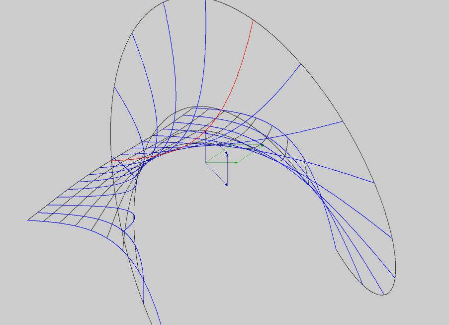
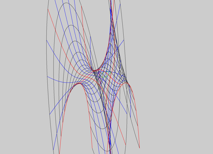
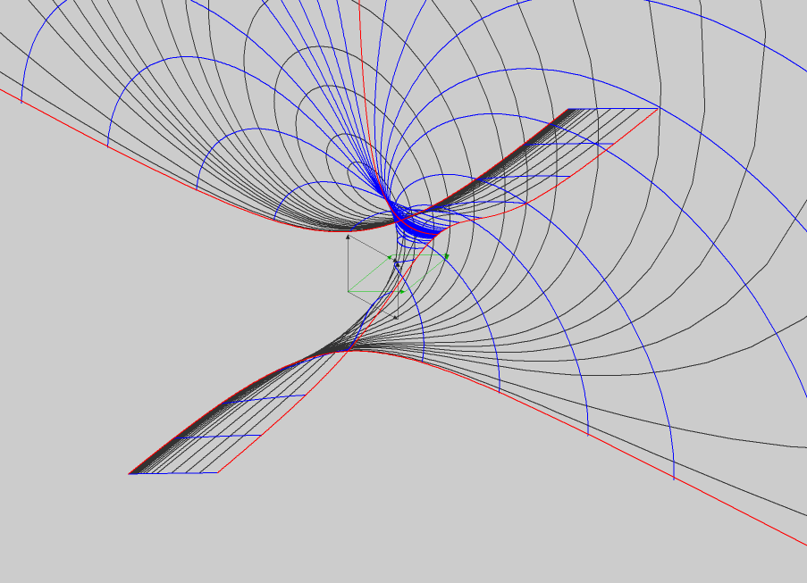
Graphing
Calculator 4.0 bis : 2D Only after rethinking
the 3D graphics of above, did I realise how it
must also be possible to use the same Graphing
Calculator 4.0 to make a 2D representation,
similar to the QBasic pictures.
The results are displayed with a flat grey
background, and may be compared with both
their 3D and QBasic analogs.
Download 2D grapher files with diverse animated
rotations (1 zip file) here.
Complex Functions
visualised
Complex planes :
Constant angle theorem This is about a nice
little theorem I discovered back then.
Just like
y = ax + b is the equation of a real Straight
line,
Y = AX + B is the equation of a Complex plane
("straight surface").
The theorem states that for any Complex plane, all
of its straight lines make a constant angle with
the X-plane. So the notion of "angle" exists in
complex space. By extension, between any two
Complex planes there exists a (consant) angle.
See video next, developing this theorem.
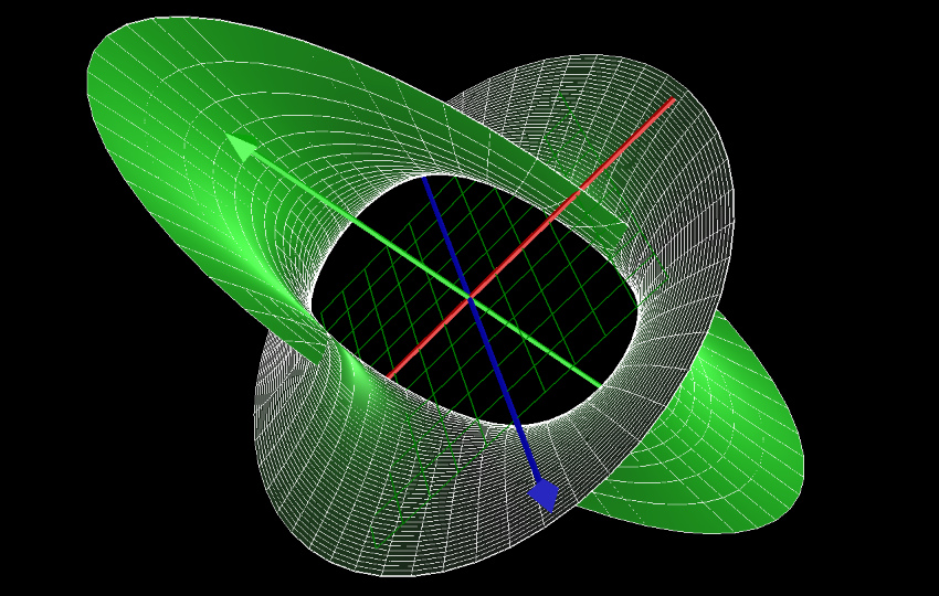
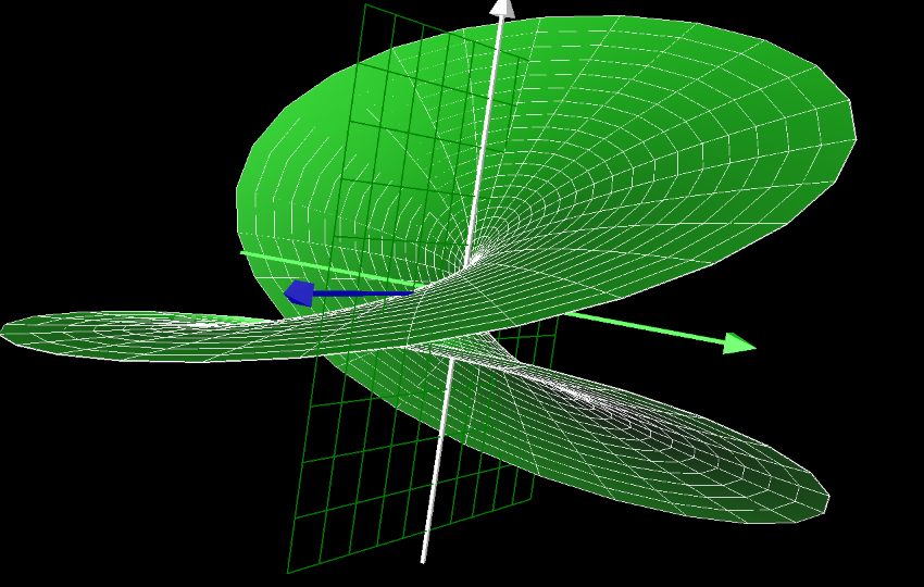
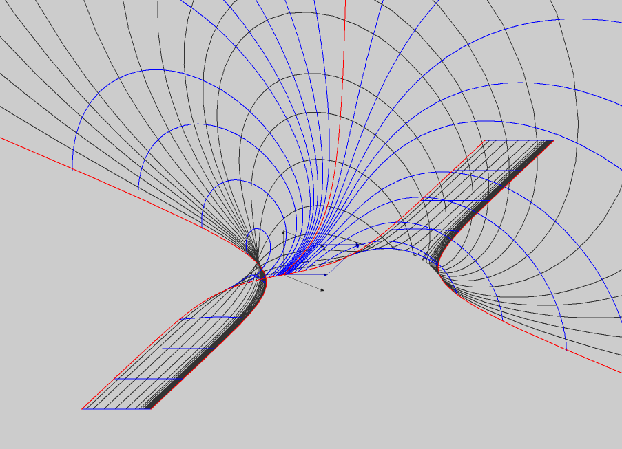
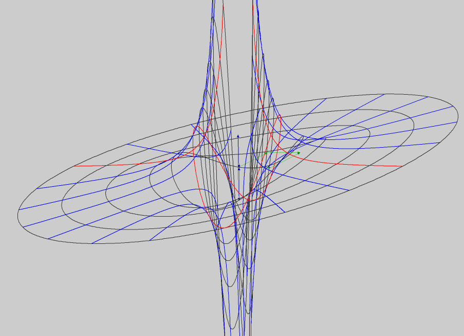
The
Circle-Hyperbola : Y = 1 / X In complex variables,
"Circle" and "Hyperbola" are the same manifold
(surface) in a different orientation. Other
"orientations":
YY + XX = 1 ; YY - XX = 1
Hence, the presence of both circle and hyperbola
curves on this surface. Notice also the two blades
extending towards the asymptotic planes, here X=0
and Y=0.
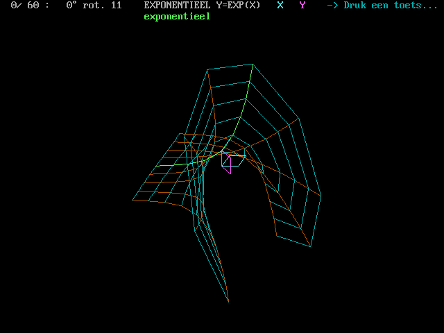
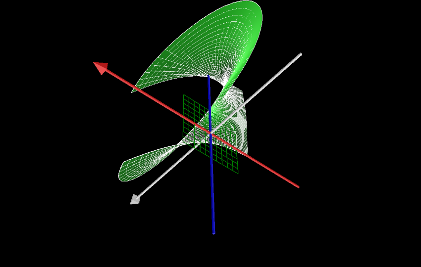
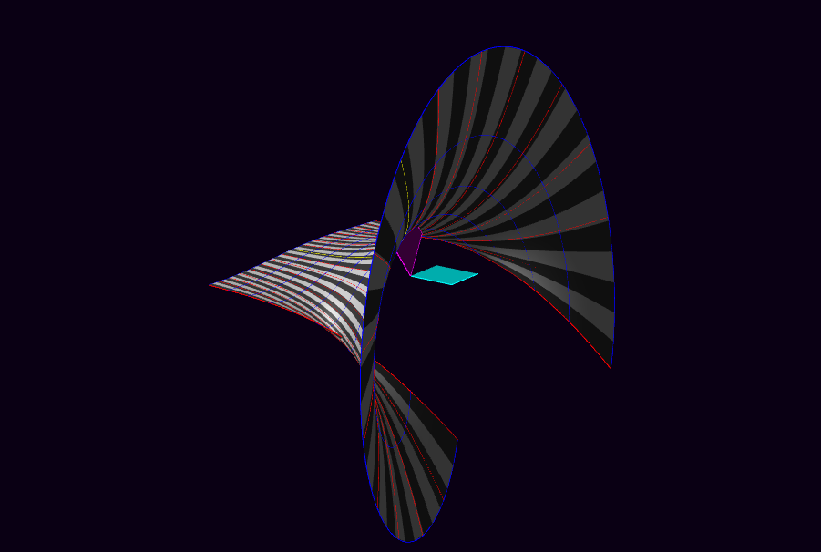
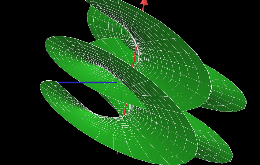
The Exponential :
Y = eX Progressive rotation
of an exponential curve, resulting in an
asymptotic blade X=0, and a screw-form blade. The
function is periodic along the imaginary X-axis
with period 2pi.
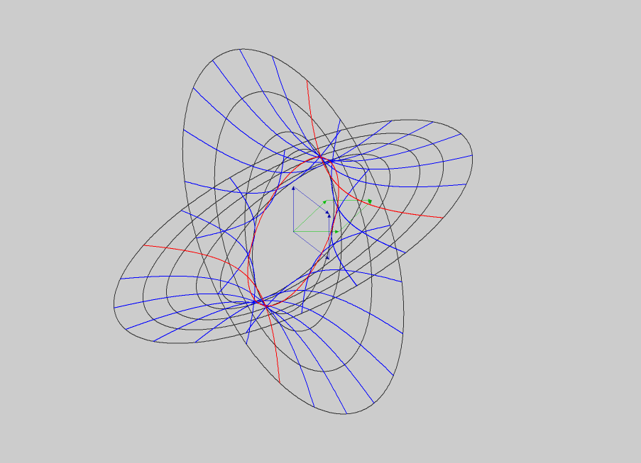
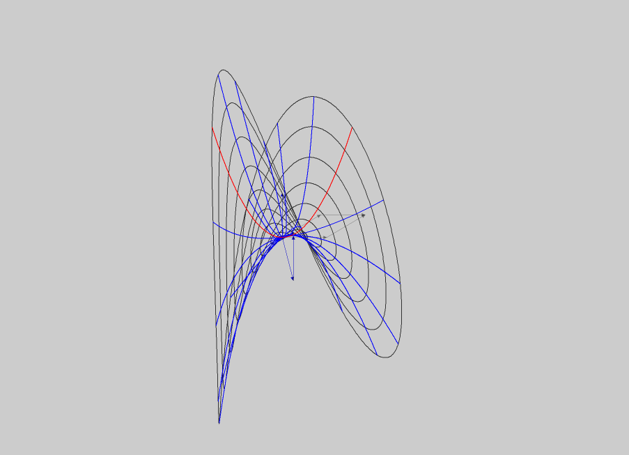
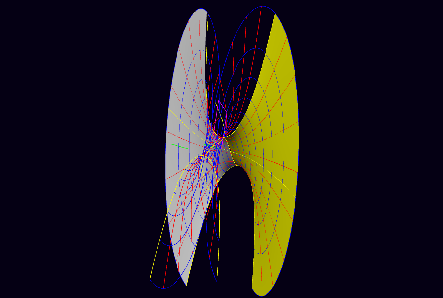
The Cosine : Y =
cos X A combination (sum
for the Cosine, difference for the Sine) of the
Exponential and its reverse. The asymptote blades
("zero") disappear and give way to a pair of screw
blades. Where both meet, the (co)sine curve
appears in the real plane, with periodicity 2p. The hyperbolic sine
and cosine are also typical curves of this
function surface.
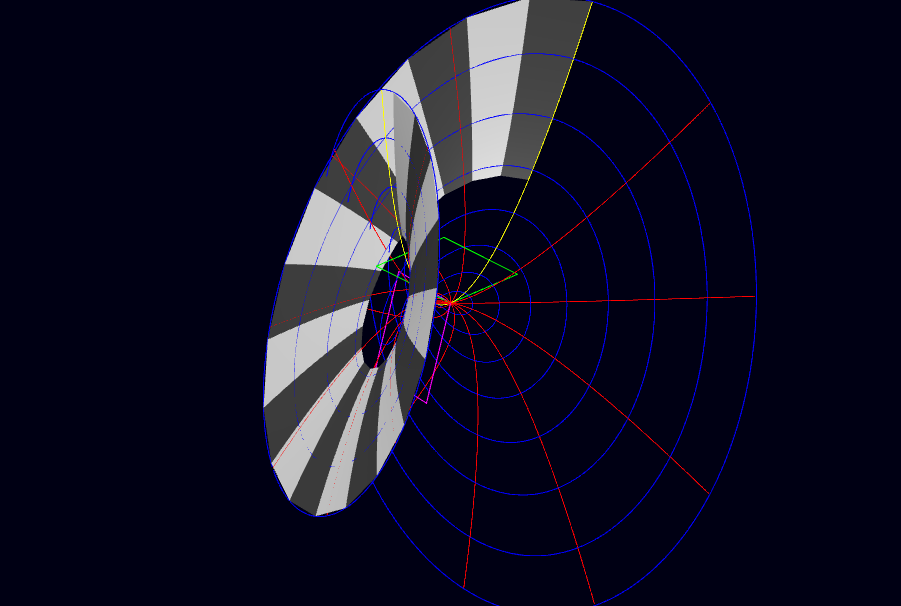
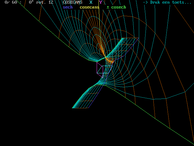
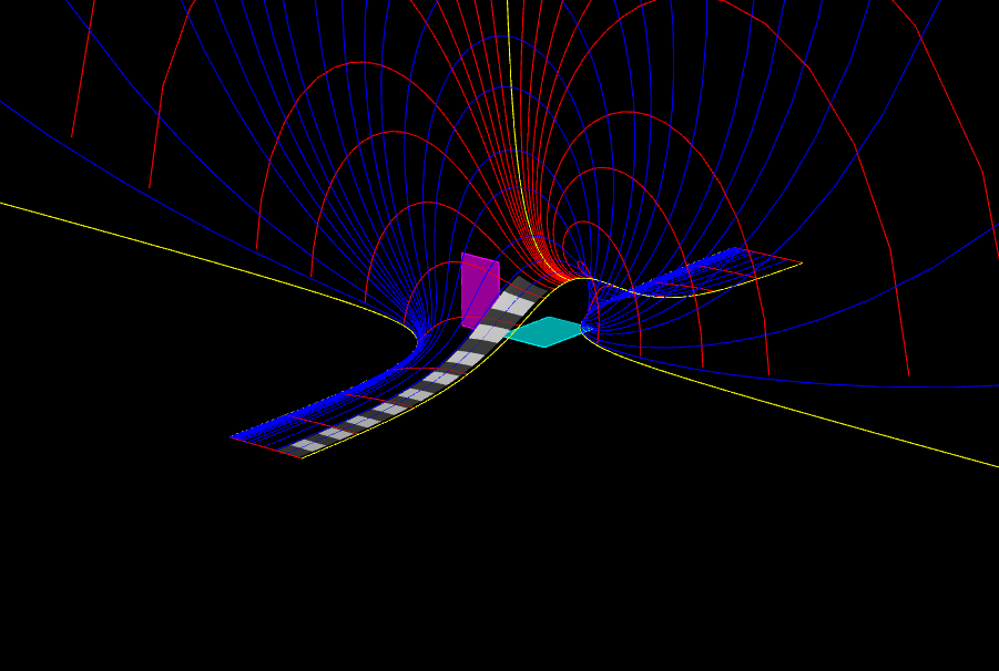
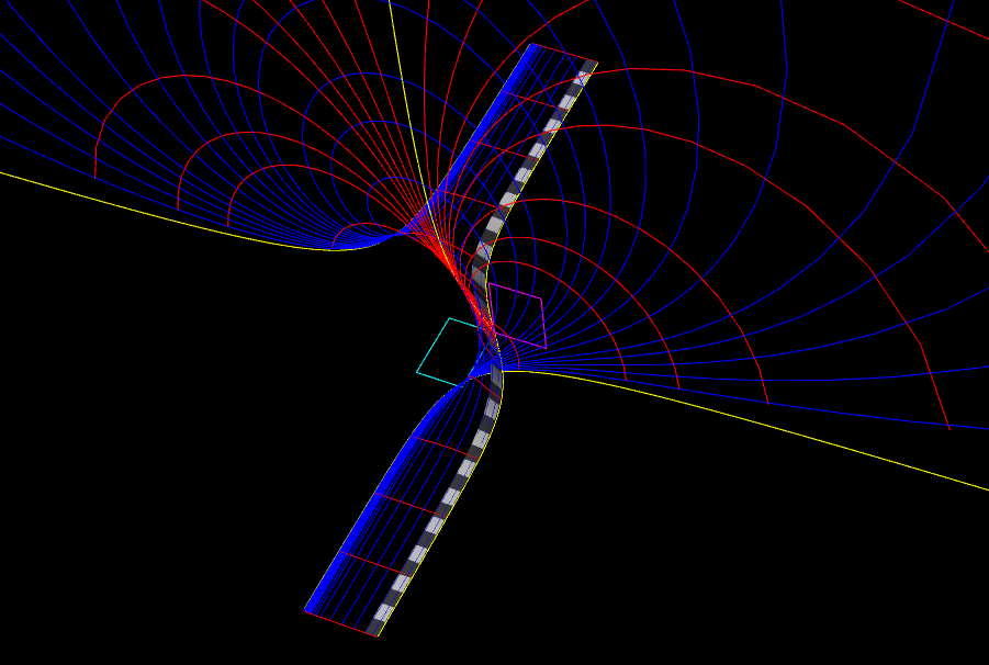
The Cosecant : Y
= cosec X A quarter of a period
of the function, with a half "up" cosec curve in
the real plane (X between 0 and p/2), and bordered by
the asymptotic planes Y=0 and X=0, by cosech
curves at one side, and a sech curve at the other.
The Tangent : Y =
tan X A half period of the
function (X between 0 and p/2), with a half tan
curve in the real plane, and bordered by the
asymptotic planes Y=0 and X=0, by cotanh curves at
one side, and a tanh curve at the other.
(A less 'fluid' gif animation here, as this item
caused an overflow bug for some rotation/step
choices in the QB-program:-)
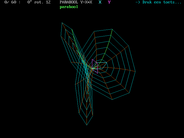
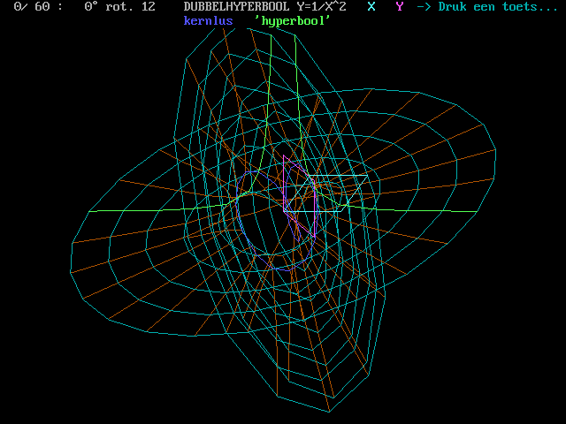
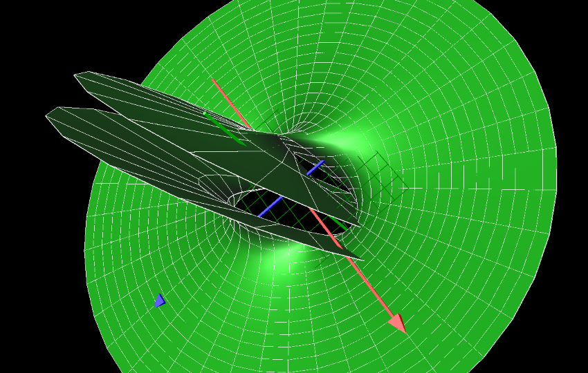
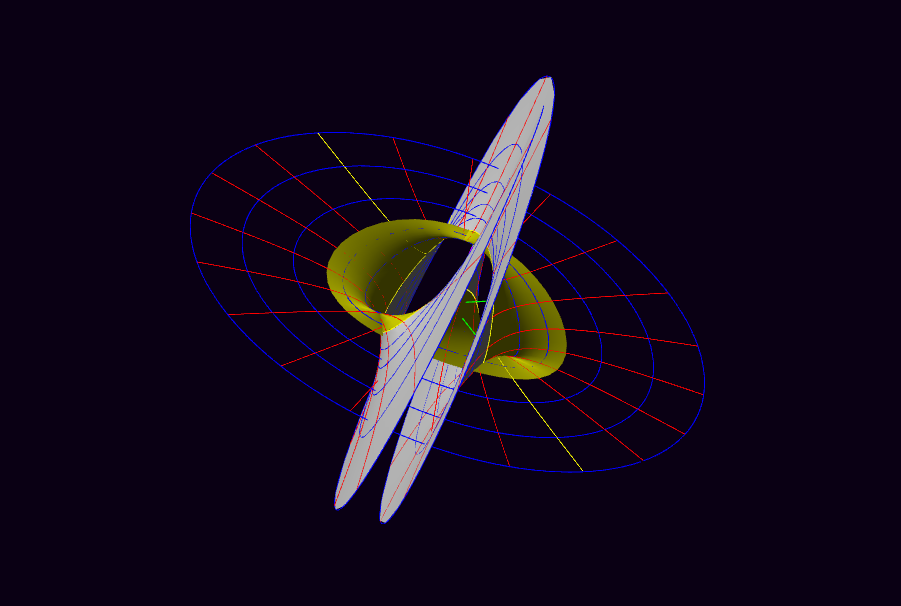
The Quadratic
Hyperbola : Y = 1 / X2 A "square"
Circle-Hyperbola, with a double bladed asymptot
Y=0, a "squared" hyperbola in the real plane and a
minimal closed centre curve somewhat like a
doublewinding circle.
This
function, z = z(x,y,u,v), concerns 5
parameters, that means, a 5D graph of a 4D
manifold.
So, generally, that would count as not
'vizualizable'.
I
proposed, however, juxtaposing two 3D graphs, by
keeping parameters constant pair-wise. That
way we'd get
fig 1: u=c, v=d; z =
z(x,y,c,d), and
fig 2: x=a, y=b; z =
z(a,b,u,v)
Then let
the "constants" a,b vary [Slider values !]
along the x,y range, and fig 2 evolve with them;
likewise,
let c,d, "Slider" along the u,v range, and fig 1
evolve with them.
This is
perfectly possible with the Graphing Calculator
4.0.
The
Graphing Calculator uses parameters xyz and x'y'z'
for twin graphs. So one should keep in mind z' =
z; x'=u and y'=v.
*****
*****
*****
*****
***** *****
Next, I realised that the same method can be applied
to two other "pairs of pairs of variables viz.
constants": z = z(x,b,u,d) and z(a,y,c,v), and z = z(x,b,c,v) and z(a,y,u,d)
Initially I achieved this by creating two more
"twin" grapher files, swapping the function
variables and constants accordingly in the formulae.
Conclusion: This function is vizualized with three
coupled twin graphs!
The drawback of this method is that each "constant"
a,b,c,d occurs in the three twin graphs, but cannot
be manipulated simultaneously to observe its
"triple" effect.
What is needed really, is a set of 6 graphs
synchronised by a single set of 4 slider values.
Unfortunately Graphing Calculator does not allow
multiple graphs beyond 2. So I thought up a trick to
at least have a demo of what I would like to see: by
off-setting the z function values for the
two remaining pairs with a z0 value (z0 = 3 in my
demo), so whereas the first pair remains at z = z +
0, the second pair is displayed at z + z0, and the
third at z - z0. That way I managed to accommodate
three graph pairs in one display pair.
Of course there is always a risk of overlap with
this system. So what I would be glad to see is
grapher software that can handle multiple graphs,
each independent but capable of being monitored by
common parameters such as sliders.
! If you know of one, better yet, if you feel like
translating this method into it, please let me
know ! ;-)
The grapher files are useable as is.
The only things to change are: redefine the function
z(x,y,u,v) and the ranges that one
wants vizualized.
Pair of coupled functions and constants.Grapher file1
In (x,y,z) : function z(x,y,c,d) and constants (a,b,0)
In (x',y',z') : function z(a,b,u,v) and constants (c,d,0)
Similar pairs forGrapher file2
, Grapher
file3
z(x,b,u,d) & (a,c,0), and z(a,y,c,v)
& (b,d,0)
and
z(x,b,c,v) & (a,d,0), and z(a,y,u,d)
& (b,c,0).
*****
*****
*****
*****
***** ***** 3 Pairs of coupled functions and constants.Grapher file In (x,y,z) : (offset values z0 = 0 ; +3 ; and -3)
function z(x,y,c,d) and constants (a,b,0)
function z(x,b,u,d) + z0 and constants (a,c,z0)
function z(x,b,c,v) - z0 and constants (a,d,-z0)
In (x',y',z') : (offset values ditto)
function z(a,b,u,v) and constants (c,d,0)
function z(a,y,c,v) + z0 and constants (b,d,z0)
function z(a,y,u,d) - z0 and constants (b,c,-z0)
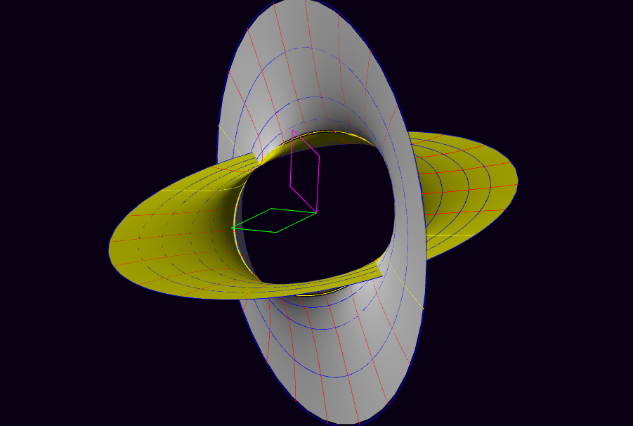
The Clifford torus evolves
in 4D space: (x,y,u,v).
The Clifford torus' coordinates
satisfy initially xx+yy=1, and uu+vv=1, so their
sum=2. In other words, it resides (also when
rotated) within the 3D shell of the hypersphere,
or "3-Sphere", with radius r = SQRT(2).
The Clifford
Torus being a 4D beast, it is often represented by a
3D projection. This is done, e.g., from the v axis
point on the 3-Sphere, i.e. v = SQRT(2), toward the
3D space (x,y,u).
Depending on the torus' rotational
position (always within its 3-Sphere), its 3D projection
Cyclide however varies from a symmetrical torus
onward, to an ever more skew one, to become an
infinitely opened surface and, beyond, reverse to a
torus but in inversed form... before starting another
half such cycle, to return to its initial form.
I wanted to show both objects, the projected and
its projection, "in the same picture". Due to the
overall 4D-in-2D rendering, both objects overlap in this
animation, whereas in 4D space they wouldn't.
The first grapher file and video show this
combination.
The (x,y,u) axes are shown in
magenta, the v axis in white, since the latter is used
as the projection origin towards 3D space (x,y,u). One may occasionally observe the
projective correspondency of the white v-axis' extremity
with the Torus' and its projective Cyclide's positions,
in their extremities...
The second grapher file and video show the
Clifford Torus only, now rotating in its 4D space
(x,y,u,v), successively along the 6 planes (u,v) - (x,u)
- (x,v) - etc.
The music is "Fraktet" - see under my muziekte.htm#Instrumentaal.
Though dating from bygone times (when I was
young:-) I discovered only recently that it is
actuelly a
"Thue-Morse sequence", fractally elongated in 3
voices. The form
is indeed a repeated theme AB-BA ... ABBA-BAAB ...
ABBABAAB-BAABABBA, etc...
See also wikipedia
: Thue-Morse_sequence
.
A sequel.
Thinking about the 3-Sphere and the special
position of the Clifford Torus in it, I then realised
that a whole family of toruses exists, which
moreover fills up the 3D space of that 3-Sphere.
These toruses have equations
xx + yy = rr and uu + vv = 2 - rr
The overall sum remains 2, so the embedding in the
3-Sphere is maintained.
The x,y circles vary their radius from 0 to SQRT(2),
when the u,v circles do theirs from SQRT(2) to 0. They
"meet halfway" with both values = 1, i.e. the Clifford
Torus.
I wanted to visualise this feature too, once again with
the "4D torus" only, and with 4D torus and 3D Cyclide
joint.
So, these are the third and the fourth grapher
files and videos...
Final remarks.
I had the impression that I had thought up some
unpublished graphic material on the Clifford and other
3-Sphere toruses, but then I stumbled into this: https://en.wikipedia.org/wiki/Talk:3-sphere
(see the projections... :-o)
Anyway, (...)
The 4D Clifford Torus and its 3D projection Cyclide
:Grapher
file1
It inspired me to these torus-less approaches to
visualise the 3-Sphere itself:
1) one by letting a sphere evolve through it along a
diameter, growing and shrinking as it marries the
3-sphere's "border", in the same way that, in 3D, a
circle would marry a sphere's border while sliding
through it; and
2) one by letting a sphere rotate within a 3-sphere of
the same diameter, in the same way that, in 3D, a circle
would rotate within a sphere of the same diameter.
! except that this being a 4D case, the plane of
rotation of the sphere would rotate, not around an axis
as in 3D, but around 2 independent axes, both
perpendicular to the plane of rotation, or in other
words, around the plane of axes perpendicular to it.
(Notice that the sphere, while rotating along the plane
of u- and v-axes, has fixed rotation points on the
x- and y-axes).